Differences in Osmolyte Concentration in Solanum lycopersicum Experiment Update

April 23, 2024

By Kylee Hanks and Sarah VanRyswyk

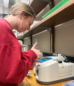
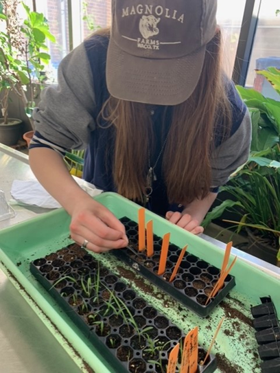
Recently in our RISEbio labs, we have been working on our research experiment. In our experiment, we were measuring the differences in osmolyte concentration in tomato plants exposed to different colored lights. Over the last few weeks, we’ve been taking osmolyte measurements from our different tomato treatment groups. There were five different pots of tomato plants under each of the three light colors. It’s been super exciting to watch our tomato plants grow and collect data to analyze, but we’ve definitely faced some large obstacles. Oftentimes, the nitrogen tank would be empty on the days we needed to take measurements. This made it hard to take consistent data every week, but we were able to get data when the tank was filled. There were other times when the osmometer would take an excessive amount of time to dry the leaf specimen. There were days we would be spending two hours in the lab to only obtain two measurements. We also ran into an issue with the leaf samples shriveling and shattering after being taken out of the liquid nitrogen.

 Despite all of the complications, we were still able to get data from the tomato plants that we could then begin evaluating. Last week, we focused on evaluating our data and working on our results presentation. We ran multiple T-tests and found that our data was not significantly different. While the osmolyte concentration data was not significant, we still saw physical changes in the tomato plants under different lights.

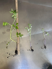
The tomato plants that had only been exposed to white lights were by far the biggest, with blue and green plants following far behind in height and leaf count. We also saw various notable observations in the way the plants had begun to grow. All 3 treatments were very etiolated, stringy, and some had adventitious roots. This was likely due to the insufficient lights and high humidity under the pots. Overall, if we were to continue this project in the future, we may experiment with different variables including physical traits, stomata data, and leaf comparisons.

Physical observation differences between tomato plants grown under white light, green light, and blue light (respectively).
Kylee calibrating the osmometer to prepare for sampling.
Posted in Plants & Environmental Stress | Tagged , , | Leave a comment

Seed germination and stomata wrap up

April 16, 2024

By Savanna Newkirk and Lily Flaherty

As the semester progressed, we continued to have numerous opportunities to improve our lab skills and gain more experience. Throughout the last couple of weeks, we have worked on guided experiments and have also created two of our own. In our last blog post, we discussed the inner workings of the beginning of our seed germination experiment. As time has passed, we have had multiple seeds germinate, meaning that we could start planting them. The first to germinate were the controlled spider milkweed (Asclepias viridis), followed by the boiled A. viridis. The wild hyacinth (Camassia scilloides) species was slower to germinate, but there were signs of germination roughly two weeks after the first A. viridis began germinating. Unfortunately, most of our sprouts died within days of being planted. In the coming final weeks of the semester, we will be analyzing our results using statistical methods.

Figure 1. Savanna planting germinated seeds.

Since our last post, we also designed and conducted an experiment that focused on the impact that drought conditions have on stomata. Our experiment involved two species of Oak, Quercus laevis and Quercus virginiana. For each species, we had two plants that we used, meaning four plants total. For each species, one plant was under drought conditions, while the other was watered well. We picked three leaves from each plant (twelve leaves total) and made stomata peels from each. We did this by painting a small strip of nail polish on the underside of each leaf, letting it dry, and gently peeling it off. We then put each peel on a slide and observed them under the microscope. We used the AmScope software to count the stomata and measure the aperture length and width. We measured the length and width of three stomata from each slide made. We have begun to analyze our results. We used a calibration slide to create a scale of pixels to millimeters, then used this scale to convert all of our data from pixels to millimeters. We also found the SPI (Stomatal Pore Index) of each slide that was made. We will continue to analyze our results by using Microsoft Excel or by coding in R.

Figure 2. Stomata from a Q. laevis peel seen through microscope and AmScope software.

We also got the opportunity to conduct a Tetrazolium test (TZ test) on cup plant (Silphium perfoliatum) seeds. A TZ test has the ability to test seeds for viability in a short time frame. To conduct the TZ test, we first acquired three cup plant seeds that had been soaking in water in order to release their hydrogen ions. Following this, we cut the seeds in half lengthwise and placed them cut side down in a petri dish with a TZ solution-soaked filter paper. The seeds were then left to sit at room temperature for 2 days. The TZ solution reacts with the hydrogen ions, staining the live tissue in the seed red while the dead tissue stays white. In all of our seeds we found that the embryo of the seed was stained red, meaning that all three of our seeds were viable.

Figure 3. Viable S. perfoliatum seeds after TZ test.
Posted in Plants & Environmental Stress | Tagged , , , , | Leave a comment

RNA Isolations, ABHD2 and DPB Sequencing, and PALD1 PCR

12 April 2024

By: Paige Hoen, Hailey Ramthun, and Mady Docteur

Figure 1. Mady working on the PCR protocol for the PALD1 samples.

Over the past two weeks, we have continued to research these three genes within the Green Anole Lizards (Anolis carolinensis): PALD1, ABHD2, and DBP. Our goal is to discover the difference in gene expression between the breeding and non-breeding season. So far, we have had more success with our primers for ABHD2 and DPB. For each of these two genes, we identified a primer set that amplifies the correct band size on a gel. With the successful primer sets, we performed a PCR clean-up and sent our samples off for sequencing. Unfortunately, we have been facing difficulties finding a successful primer set for PALD1.

Figure 2. Gel image of RNA Isolation for a liver sample.

After numerous trials and errors with our first three primer sets for PALD1, we concluded it would be best to design new primers. When our new PALD1 primers arrived, we reconstituted them by adding water. Then, we performed PCR using each new primer set. After the PCR was completed, we loaded each sample into a gel and imaged it to see if the correct band sizes for each primer were amplified. Our results from the gel image showed primer dimers for two of the primer sets, and the other primer set showed hardly any bands. This means that we will continue troubleshooting with these primer sets. While working on PALD1 primers, we received our sequencing for DBP and ABHD2. The sequencing showed that our primer sets for both genes are good. Along with working on PALD1 primers, we have spent the past couple of weeks practicing RNA isolation. Eventually, a future step of our project is to perform a qPCR to analyze gene expression. We will need decent RNA isolation samples to complete this. The protocol for RNA isolation is slightly more complex than some of our previous protocols. This is because the RNA in the tissue can degrade if we do not work quickly enough. To practice with this protocol, we began by using liver samples in our first two attempts at RNA isolation. This was to make sure we knew what we were doing before using a brain tissue sample. After doing RNA isolation with liver tissue, we loaded our sample into a gel and imaged it. Both gel images showed that our RNA isolations were successful; showing two dark bands.

Figure 3. Paige and Hailey imaging the gel.

Since we successfully performed RNA isolation on liver tissue, our next step was to perform it again using brain tissue. Brain tissue thaws faster than liver tissue, so it was important that we worked quickly during the protocol. We completed our first brain sample RNA isolation. When we tested our sample on the Nanodrop, we got a concentration of 255.5 ng/µL along with a purity of 2.12. Purity should be close to 2.0, so we were pleased with these results. We ran a gel with the same sample. The gel showed two bands; therefore, we completed the RNA isolation successfully. We did another RNA isolation using brain tissue, and it had good concentration and purity. Next week, we will run a gel using this sample.

Our next steps for the remainder of this semester are to complete two more RNA isolations with a brain sample, ensuring we are consistently successful. Along with this, we will continue troubleshooting PCR for our three PALD1 primer sets. We will try PCR with a dilution, or a temperature gradient, to discover an effective PALD1 primer. An effective primer will amplify the correct band size in a gel electrophoresis with little to no primer dimers. Once we find a primer set that works, we will perform PCR cleanup on it and send it out for sequencing. Overall, we have made a lot of progress these last few weeks in the RISEbio lab. We have found two working primer sets, successfully performed RNA isolations, and are troubleshooting new PALD1 primers. These past weeks have not only taught us new lab skills, but the importance of staying on track, using time effectively in lab, and moving quickly to complete our tasks.

Posted in Brain & Behavior | Leave a comment

Drought Experiment with Q. buckleyi

9 April 2024

By Ash Waletski and Katelyn Gianni

As the spring semester comes to a close, we have mainly been working on our longest and most detailed experiment so far. Since our last update, we planned and designed an experiment focused on the chronic effects of drought. We chose to work with Quercus buckleyi, the Texas red oak, because it is a close relative to Quercus rubra, the very common Northern red oak that is native to Minnesota (there’s actually a few of these on our campus!). We figured our findings would be more transferable to local ecosystems if we chose an oak species genetically similar to those found nearby.

We want to see if Q. buckleyi saplings that have already acclimated to low water availability, like drought, would have differences in their abilities to uptake water once drought periods are over. We designed our experiment with three groups of five Q. buckleyi saplings each, to control for as many variables as possible (Figure 1). The original states of each group have been maintained for three years in the biology department’s greenhouse, and we changed watering conditions and moved saplings around accordingly about four weeks ago (Figure 2). We had some difficulty moving the saplings that have been grown under well-watered conditions though– they kept getting stuck because of their well-developed roots.

Figure 1. Visual guide for the groups and treatments used.

Every Wednesday since then, we have been looking at the volumetric moisture content left in the saplings’ soil, with the long-term goal of seeing how saplings’ water uptake has been affected. We have been taking and recording percent moisture in each sapling’s soil using a soil moisture sensor (Figure 3). Later this week, we will be diving into another way to see how the saplings have been affected by release from drought– finding specific leaf area, which is the ratio of leaf area to leaf dry mass.

Scientifically, there is a well-documented relationship between a plant’s specific leaf area and the amount of photosynthesis that’s going on inside it; essentially, the denser the leaf, the less photosynthesis it’s able to do. Photosynthesis requires water, so if our experimental group of saplings have different specific leaf areas to either control group, it could be indicative of a change in water uptake. It’s been absolutely fascinating diving into the primary literature behind these processes and learning all about what’s going on inside our little oak saplings. Time and data will tell!

Figure 2. Katelyn rearranging hoses to change watering conditions.

            In the meantime, before we start calculating specific leaf area and between the days that we measure soil moisture, we have been practicing statistical analysis and wrapping up our previous seed germination experiment. Overall, this drought experiment so far has been going quite well and has been a great learning experience. It’s especially been exciting learning new lab techniques. As we mentioned earlier, moving forward our next steps are to calculate specific leaf area, then perform statistical analysis with those values and also with our full soil moisture data. We are very excited to present our future findings to our entire RISEbio team!

Figure 3. Ash measuring soil moisture content using a soil moisture sensor.

Posted in Plants & Environmental Stress | Tagged , , , , | Leave a comment

ADAM9 and BHLHE40 PCR Clean-Up and RNA Isolations

5 April 2024

By: Arya Haala & Elenore Milde

Figure 2. Arya and Elly working on RNA isolations.

Since our last update, we chose two genes to research, ADAM9, and BHLHE40, and designed three primers for each gene. We continued our work with PCRs and gel electrophoresis by adapting them to fit our unique needs. Most notably we worked with a temperature gradient to find the temperature our primers worked best at. As research continued, we threw out two primer sets from each gene, keeping the most effective one for each.

During trouble shooting we used PCR and gel electrophoresis to get clear bands at the correct amplicon size. The size was based on the region of DNA the primers amplify. Once we got the seemingly correct amplicon, we started PCR cleanup to isolate the additives from our gene amplicon. To do this we used 10 μl of our PCR samples and ran a gel to ensure our samples were good. After we confirmed our band sizes were a match, we began our PCR cleanup so we could send out a clear sample for sequencing. We used the remaining ~15 μl of our mixture and 5 volumes of DF Buffer in a column. Centrifuging it and adding 15 μl of Elution Buffer before centrifuging it again. We used the Nanodrop with 1 μl of our solution to measure the DNA concentration and purity of ~1.8. Our purity was a little low, but we continued. We used C1V1=(1 ng/μl)(15 μl) to determine the amount of water needed for sequencing. When this was done, we added the solution, calculated water volume, and 1 μl of the genes forward primer to a PCR tube. This was then sent out for sequencing.

Figure 1. Gel image of temperature gradient

When the samples came back from sequencing, we used the 4Peaks software to analyze our data. Our results came back with a 100% match for ADAM9 and a 95% match for BHLHE40 in the NCBI database. This led us to put the primers away for future use before moving to RNA isolations.

We did two practice RNA isolations on liver tissue to ensure we are ready for real brain tissue. To do this we took one third of a frozen liver sample collected from green anole lizards and homogenized it with 1 ml QIAzol to stop the RNA from degrading. That sat for 5 minutes, then we added 200 μl of chloroform and vortexed. It sat again for 2 minutes before centrifuging at -4°C for 15 minutes. After the 15 minutes was up, we had three layers: clear, white, and red. We pipetted the top clear layer into a new tube getting approximately 600 μl, then added the same amount of 70% ethanol and vortexed to mix. Then we added this new mixture into a column, discarding all flow through. We added 350 μl Buffer RW1 and centrifuged twice then 500 μl Buffer RPE and centrifuged twice more. Following this we used 30 μl of RNA-free water and centrifuged two times using the same water. After this was complete, we used 1 μl of our RNA solution and the Nanodrop to test the concentration and purity.

Both of our liver tissue samples had an ideal purity of ~2 and a concentration that was good for the mass of tissue. Because our samples worked, we used a gel to determine if our RNA had band sizes at 185 and 285 base pairs. Through gel imaging, we determined our samples had good band sizes. Since both of our practice samples went well, we started our first RNA isolation using brain tissue. The difference between brain and liver tissue in RNA isolation is now you will add two steps in the protocol using DNase to make sure all DNA has been transcribed into RNA.

Posted in Brain & Behavior | Leave a comment