PCR, Gel Electrophoresis, and qPCR for ABHD2, DBP, and PALD1

By: Mady Docteur, Paige Hoen and Hailey Ramthun

11 October 2024

Figure 1.A gel showing all our genes: PALD1, DBP, and ABHD2, and Beta-actin.

This semester, we have continued to research our three genes: ABHD2, DBP and PALD1 and how they are expressed in green anole lizards (Anolis carolinensis). The goal of this research is to see gene expression differences between the breeding and non-breeding seasons of the lizards. Last semester, we found a successful primer set for both ABHD2 and DBP. We also found three successful primer sets for the gene PALD1.

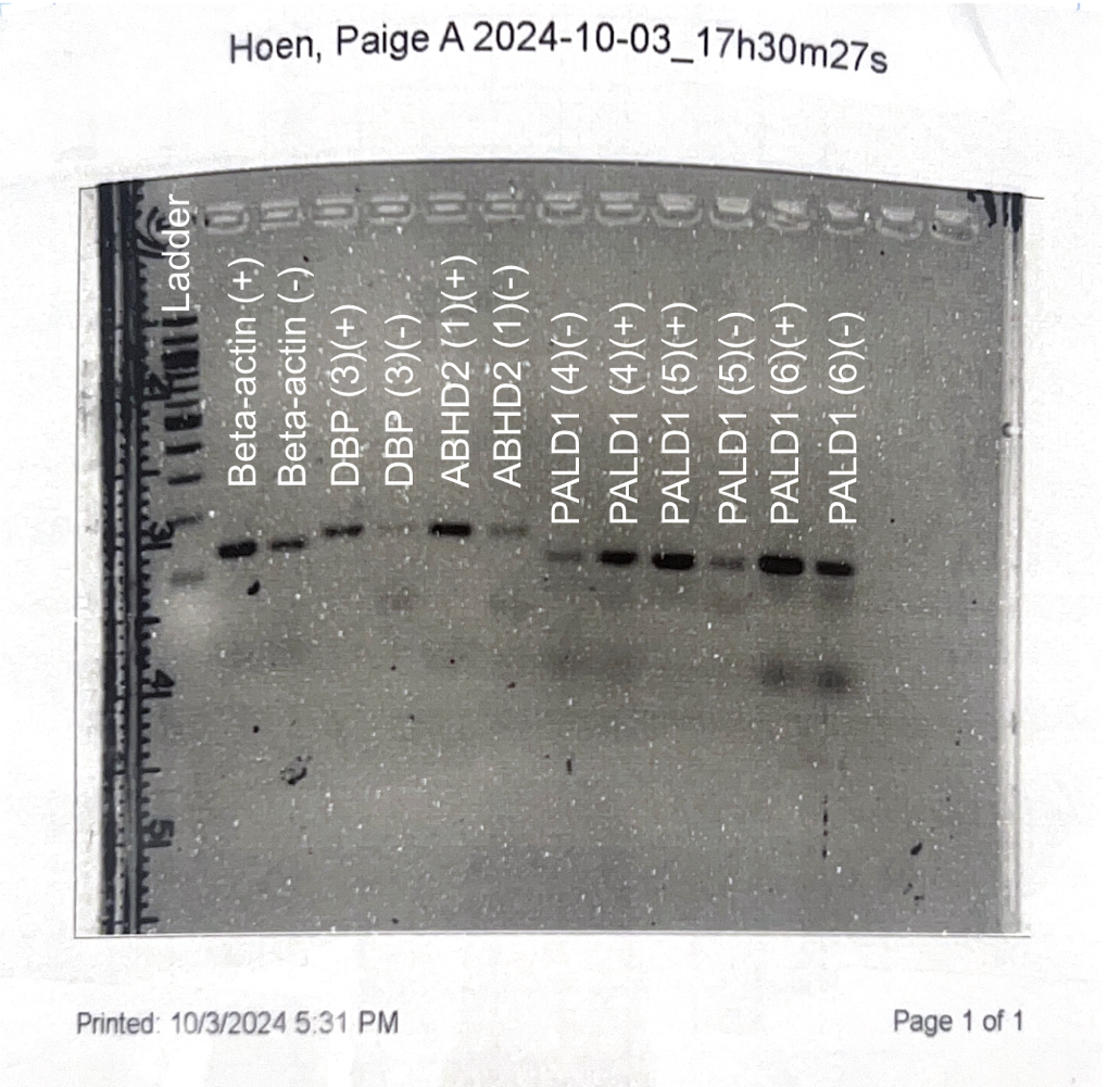
In the past two weeks, we have been ensuring all these primer sets still work through PCR and gel electrophoresis. After performing gel electrophoresis, we image each gel to check that the correct band size is amplified for each primer set. In our last gel image, all our primer sets amplified the correct band size; however, a lot of primer dimers were present. Although primer dimers are not ideal to have in a gel, we decided to move on to qPCR.

Last week, we set up a qPCR for the first time. The difference between qPCR and PCR is that qPCR allows us to monitor a PCR reaction in real time and receive more detailed results. When setting up a qPCR, we create multiple serial dilutions of a master mix to create a standard curve. Then, we load each dilution into a 96-well plate.

 After loading the plate with our samples, we perform the qPCR software protocol. We start by setting up our experiment on a computer to collect data. In this data, an important value we look for is our PCR efficiency for each primer set. Unfortunately, our qPCR showed PCR efficiency values that were much higher than they should be. This could be due to primer dimers or pipetting error when setting up the qPCR.

Figure 2. Hailey, Paige, and Mady preparing the qPCR software to run samples.

After running our qPCR plate, we performed gel electrophoresis and loaded each of our samples into a gel. After imaging the gel, it showed numerous primer dimers. This could have been due to inaccurate pipetting or adding contaminated cDNA when preparing the qPCR samples.

Our next step will be setting up another qPCR. We will use different cDNA to try to limit primer dimers and focus more on pipetting carefully. We are hoping to end with a lower PCR efficiency value. If the results of our next qPCR are not what we are looking for, we will begin troubleshooting. The past couple of weeks have taught us that research does not always go smoothly. Results do not always come back how we want them to, but this allows us to practice perseverance despite challenges and learn troubleshooting skills.

Posted in Brain & Behavior | Leave a comment

Turning over a new leaf: exploring proline and project plans!

By: Ashley Waletski and Katelyn Gianni

We have just started our second-semester RISEbio project! We are still observing the impacts of drought stress on Quercus (oak) saplings, but this time, using some new metrics, and a different species, Q. agrifolia. We learned an exciting new lab technique to use in our experiment – finding proline concentrations in leaves. Proline is an osmolyte produced by plants when they are under stress (like drought, which we are studying). Proline in freeze-dried and pulverized leaf tissue reacts to ninhydrin, a chemical we add, forming a red hue; the deeper red, the more proline present. This red color can be quantified using spectrophotometry, after which we can plot points on a graph in relation to known proline values, to figure out exactly how much proline was in that leaf. Here (in Fig. 1) you can see test tubes of leaves we sampled, in a container of liquid nitrogen, being prepared to be freeze-dried. We haven’t quantified proline quite yet for the experiment with our own Q. agrifolia specimens, but we spent time last week preparing leaves to do so (Fig 2).

Figure 1. Katelyn putting a test tube of fresh leaves into liquid nitrogen. This helps prepare the samples to be freeze-dried.
Figure 2. Ash placing Q. agrifolia leaves into a test tube. See our specimens in the background with the pink tags!

Another new metric we learned and examined between our mesic and xeric groups this week was leaf dry matter content (LDMC), which is a measure of how much of a leaf’s mass is water weight, and how much the actual leaf tissue. LDMC is calculated as the ratio between the mass of a freshly picked leaf and the mass of that same leaf when dry. To find this, we plucked one leaf per sapling, weighed and recorded each leaf’s mass, dried the leaves out in a drying oven, then weighed them again to find that dry mass. Additionally, separate from LDMC but using this same data, we found how much weight in the fresh leaves was due to water content. Fascinatingly, this averaged 39.9% for mesic and 40.5% for xeric (that’s a lot of water!).

Also during this past week, we submitted proposals for institutional undergraduate research grants – this semester, in addition to and inspired by our RISEBio work together, the two of us decided to start separate independent study projects. These individual research projects will build our research skills even more, especially through reading lots of primary literature, which will strengthen the work we do in RISEbio too.

It’s been a great start to the semester with lots of new experiences for us! Whether it be designing this experiment, learning lab skills like proline quantification, learning more functional traits like LDMC, or exploring even more research, everything has been so exciting.

Posted in Plants & Environmental Stress | Tagged , , | Leave a comment

The Beginning of Quantifying Proline

By Sarah VanRyswyk and Kylee Hanks

Recently in RISEbio, we have been quantifying proline using a colorimetric assay and practicing making a standard curve via spectrophotometry using a 96-well plate.

Proline is an amino acid that plays a key role in stress response in plants. It can accumulate over time and high levels are an indication of high stress. In our experiment, we used a colorimetric assay with spectrophotometry to determine the proline concentration in several different oak species.

To begin this process, we selected 100 mg of leaf tissue from two different oak species. The species we chose were Q. macrocarpa grown in well-watered conditions and Q. rubra grown in drought conditions. We then proceeded to grind them up into fine powders, removing primary and secondary veins from the powder. Next, we prepared our seven standard solutions (46, 36.8, 27.6, 18.4, 9.2, 4.6, 0 μL/mL).We pipeted the appropriate volume of the standard solution into each of our test tubes and then pipetted the corresponding amount of water into the test tubes as well.

Under the fume hood, we pipette 1000 μl of 3% sulfosalicylic acid to our leaf tissue samples. We then stirred these with a metal needle until the two were completely mixed. Next, the samples were centrifuged for 5 minutes and placed onto ice immediately after. To prepare the test tubes, we added 100ul of 3% sulfosalicylic acid, 200 μl glacial acid acetic acid, and 200 μl of acidic ninhydrin to each test tube including our standards.

After taking our leaf samples from the ice bath, we pipette 100 μL of the supernatant, a liquid that lies above the settled leaf residue in the test tubes,  from the top of the tubes into our leaf tissue test tubes that we had prepared. Next we pipette 100 μL of each sample and standard into their appropriate wells.

Finally, we had the well plate read by a spectrophotometer and then analyzed our results. Q. macrocarpa had a proline concentration of 39.12 (μL/mL), while Q. rubra had a proline concentration of 50.13 (μL/mL). It was expected that Q. rubra would have a higher proline concentration, as it is under more stress from being grown in drought conditions. Overall, this project was super interesting and pretty straight forward! From this experience, we learned a new skill of quantifying proline from leaves and how to interpret the concentration values we get. We plan to dedicate our research this semester to comparing proline concentration in various Ozark Oak species, as Dr. Kaproth found 8 species located in the same area. We plan to look at the different species samples and analyze what differences we find in proline concentration, lobe shape, and leaf area.

We are excited to get back to work this semester and begin a new research project!

Figure 1. Kylee and Sarah pipetting the proline for the standards.
Figure 2. An example of the leaf grinded into powder to prepare for proline quantification.

Posted in Plants & Environmental Stress | Tagged , , , | Leave a comment

Proline Quantification

By Wren Poessnecker and Logan VanGuilder

To begin this semester of research we were introduced to proline quantification. Proline
quantification is the process used to find the amount of the amino acid proline is in a given
sample. Proline in plants acts as an osmolyte and tends to be created while plants are
experiencing abiotic stress. We performed a colorimetric assay to quantify the proline present in two plants.

For the first week of protocol, we created a standard curve using distilled water and red
food dye to get used to the process. Later in the week, we spent some time grinding tissue using a mortar and pestle for our two plants to be used as our tissue samples the following week.

The next week was the real run-through. From our ground tissues, we selected three 100
mg samples from each of our two species. We created a standard curve of proline by doing a
dilation of the proline standard and distilled water. The concentrations of proline measured to
create the curve were 46, 36.8, 27.6, 18.4, 9.2, and 4.6 μL/mL. To each of our tissue samples, we added 1000 μL of 3% sulfosalicylic acid and mixed it together with a pin. This took a lot more time than we expected, and for this protocol, time was very important, so it’s a good thing we had some practice from the previous week to speed things along. Next, we needed to separate the tissue from the supernatant by placing the samples into a centrifuge for 5 minutes.

Standard Curve of our water practice.

Some of the samples were difficult to separate, so we had to do a couple runs through the centrifuge. To each of our 21 standard test tubes and 6 sample test tubes, we added 100 μL of 3% sulfosalicylic acid, 200 μL of glacial acetic acid, and 200 μL of acidic ninhydrin. To our sample test tubes, we took 100 μL of supernatant from each of our tissue samples and placed it into their respective tube. To finish off the test tubes we placed them in a hot water bath of 96 °C for one hour. We then pipette 100 μL of each sample into a 96 spot well plate following the plate map. After that, we inserted the well plate into the spectrophotometer and ran the program at 520 nm. Leaving us with the data in an Excel spreadsheet we turned it into a standard curve. From there we measured the concentration of proline based on the value of the line of best fit, finding that Sample 1 had a concentration of 55.0 and Sample 2 had a concentration of 64.5.

The difference in concentration between our two species gives us a good idea about
different plants’ ability to react to abiotic stressors. In this protocol, we saw the proline
concentrations of two plants, and in the future, we could see the concentration in many more
species to see how proline compares to other drought response factors, such as stomata size and density.

Standard curve including our two samples (red dots) and their proline concentrations (μL/mL).

Posted in Plants & Environmental Stress | Tagged , , , | Leave a comment

CDNA synthesis and qPCR practice

By: Sarah Oberstar and Kaity Shaffer

24 September 2024

Kaity is pouring agarose into a flask.

We are back in the lab, ready to continue our research from last spring. In the final weeks of the previous semester, we finalized and sequenced our primers for KCNJ4 and NR1D2. We also finished isolating RNA. This semester we are using our isolated RNA and turning it into cDNA. We are also preparing to take the next step in our research, qPCR. This includes practicing standard curves and serial dilutions. 

We started by converting our isolated RNA to cDNA through cDNA synthesis. RNA is very unstable and must be stored at –80 degrees Celsius. By converting RNA to DNA, it becomes much more stable. We don’t have to store it at such low temperatures, and it becomes easier to work with. In total, we synthesized six different samples for the research stream to use. After all six samples were converted into cDNA, we performed a PCR using a primer we know worked and gel electrophoresis to make sure that the band sizes looked correct. This makes sure we have quality cDNA to use for future experiments. We have done this process twice, so far five out of the six samples have turned out well. 

Sarah is pipetting the DNA ladder.

The next step in our research will be qPCR. This week in the lab we just practiced the protocol using water and dye. We started by making a serial dilution. We used three tubes to make our concentrations. Each tube was more diluted than the last. This series will be similar to the one we will use to make a standard curve for when we do the real qPCR. Next, we did some dilution calculations just to make sure we understood the math. Lastly, we practiced the qPCR protocol. In the past we have used microcentrifuge tubes to do PCR, this time we got to use a 96-well plate. Each of us got a map and used colored water to fill said plate. This was a very cool practice to do, we are very excited to do the real qPCR. 

All in all, we synthesized cDNA from RNA and verified its quality using PCR and gel electrophoresis. Five out of the six samples have so far been successful. We need to keep working on the last sample in the coming weeks. We practiced the qPCR protocol and are looking forward to applying it in future experiments. We learned many new things about qPCR, the protocol, and the process. We learned that we will have to be patient and focused when completing the real protocol. We discovered how serial dilutions and standard curves relate to qPCR.

Posted in Brain & Behavior | Leave a comment