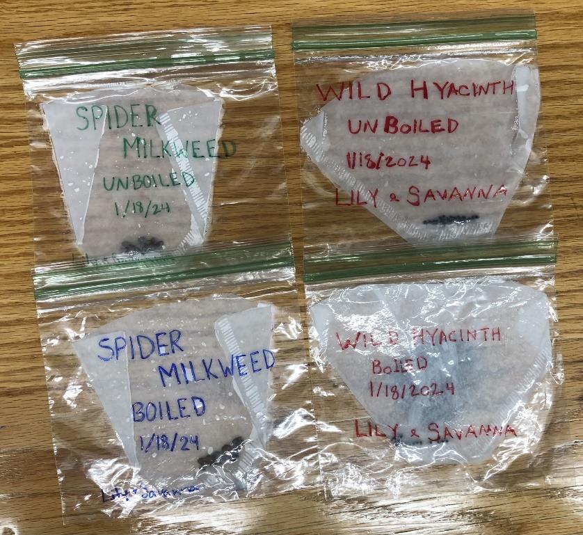
We began the semester by designing and conducting our seed germination experiment. To begin the experiment, we chose two seed packets out of a selection of native Minnesotan plants. The seeds we chose were that of the spider milkweed (Asclepias viridis), which has a germ code of C30 and the wild hyacinth (Camassia scilloides), which has a germ code of M. Seeds with a germ code of C30 need to germinate in a cold, moist environment for 30 days before being planted, and seeds with a germ code of M are best planted outdoors in the fall.
For our experiment, we followed the steps for germ code B with half the seeds from each packet, 24 seeds for the spider milkweed and 44 seeds for the wild hyacinth. For germ code B, you pour boiling water over the seeds and then leave them to soak in the water for approximately 24 hours. Due to scheduling, we allowed the seeds to soak for two days instead of 24 hours. After letting the seeds soak, we followed the steps of germ code C30 for all of the seeds, placing the seed groupings, one group of the germ code B treated seeds and one untreated from each plant, into a coffee filter and dampening it with distilled water before placing it in a sealed plastic bag and allowing them to germinate in the refrigerator. Our hypothesis was that the boiling water would negatively impact the seeds of the spider milkweed, while the wild hyacinth would benefit from the treatment.
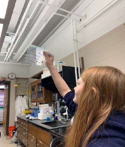
We checked every week for any changes to the seed groupings, as well as changing the coffee filters as needed to prevent mold growth. However, no changes have been noticed thus far.
Figure 1: Seed Germination Groups
Figure 2: Savanna Observing Seed Group
We also had the opportunity to measure stomatal densities and aperture lengths. Stomata are small pores in plant tissue that allow gas exchange to occur, which is necessary for life. Aperture lengths are the lengths of the open pores. By learning about this information, we were able to determine how plants and their stomata characteristics help them survive in their environment.
For our experiment, we chose two species of leafy plants from the greenhouse here at MNSU to measure. The first species we chose was a weeping fig (Ficus benjamina), and the second species was an angelwing jasmine (Jasminum nitidum).
To begin the process, we picked three leaves of each species. We then painted a small strip of clear nail polish onto the leaves. We were careful to avoid large, prominent veins. We tried to avoid the veins so that our samples would have an accurate stomata count, as veins do not contain stomata. After leaving the paint to dry, we took a piece of clear tape and attached it to a small part of the nail polish. We slowly peeled the nail polish off the leaf – carefully so that we did not touch the polish – and placed the polish on a slide. After sticking it to a slide, we secured the sample by using more tape. We were then able to observe the stomata through a light microscope.
Through the microscope, we were able to count the number of stomata that were seen in a given area. We took the averages of all three samples of each leaf and found the densities for both species. For our first species, – Ficus benjamina – the leaves had an average stomatal density of 143.543 stomata per mm² and an average aperture length of 0.03630 mm. For our second species, – Jasminum nitidum – the leaves had an average stomatal density of 276.018 stomata per mm² and an average aperture length of 0.04720 mm. After several other calculations, we determined that the SPI (stomatal pore index) for the Ficus benjamina was 0.18915 mm². We also calculated the SPI for the Jasminum nitidum and obtained a result of 0.61492 mm².
In the first month of our research stream, we have already done three separate experiments. Those experiments have been seed germination, stomatal pore measuring, and osmosis labs.
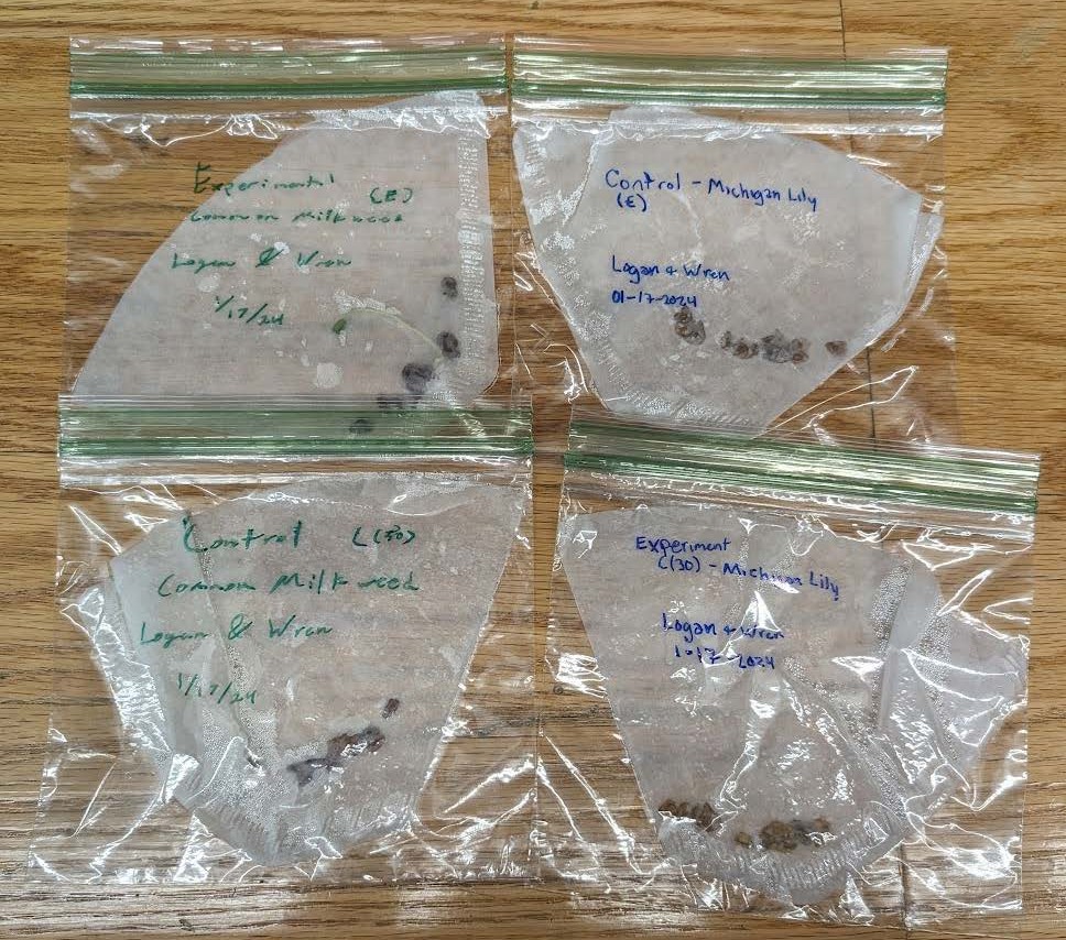
To begin the semester we started by working on a seed germination experiment. We began by choosing which of the common germination codes we would be experimenting with. The ones that we chose to go with were germination codes C30 and E germination code C30 has the seeds germinate in cold moist areas for four weeks, while germination Code E calls for 2 weeks in a moist warm environment followed by two weeks of a cold moist environment. We chose one plant that is traditionally a C30, common milkweed (Asclepias syriaca), and one plant that is traditionally an E, the Michigan lily (Lilium michiganense). We are testing how both plants respond to both environments. Our hypothesis is that both plants will respond better in their native environment. We are testing this by putting 15 seeds per plant per germination code in a wet coffee filter. We then put each in a separate ziploc bag and put them each in their germination code situations. Each week we check for growth and abnormalities. The first week we found large amounts of mold on the E plant seed’s coffee filter but after changing the filters it never happened again. So far two weeks have passed and only one seed has begun to grow, a seed from the E germination of the common milkweed. This result was highly unexpected considering it is typically grown in a cool environment and we had it in a warm environment at the time it began to sprout.
Current progress of our seed germination experiment.
We started our second experiment about the stomatal pore index (SPI) of different plants on January 24th, and finished it on the 29th. The purpose of this experiment was to help us understand how the SPI of different plant species varies based on their climates. Since the stomata of plants is used for gas exchange as well as the expulsion of water, the SPI of a plant can tell us a lot about how it has adapted to live in its environment. We started the experiment by selecting 3 leaves each from 2 different species in the greenhouse that we expected to have variation in their SPI.
The 2 species selected were Tradescantia pallida (purple queen spiderwort) and Geranium robertianum (herb robert). T. pallida can be found in eastern Mexico, it has large, smooth, and thick leaves with a deep purple color. G. robertianum is commonly found in Europe, but can also found in other parts of the world. It has much smaller leaves that are thin, hairy, and green. After gathering our leaves, we began the process of gathering leaf peel impressions. We painted the underside of each leaf with roughly 1 square centimeter of nail polish. Once the nail polish dried, we used tape to peel it off and attach it to slides. We had few issues getting the impression from the T. pallida leaves, but the G. robertianum leaves were too thin and hairy to successfully peel the impression, so after attempting to shave off the hair, we waited for the nail polish to dry more while examining T. pallida under the microscope. Using the microscope, we examined the number of stomata in an area and the average length from 3 separate stomata for each leaf.
Across the 3 leaves of T. pallida, they had an average count of 9 stomata with an average aperture length of 0.0524 mm. As we were running out of time and the G. robertianum impressions were not peeling correctly, we wrapped up for the day.
We continued the experiment on January 29th by selecting a new plant from the greenhouse to replace G. robertianum. The plant selected was Querus virginiana (southern live oak). The leaves we gathered from Q. virginiana were small, smooth, round, and green. To get an impression from these leaves we followed the same process as before with the nail polish, but we had a much easier time with this plant. Under the microscope, we found an average of 619 stomata with an average aperture length of 0.0103 mm. For each species we followed a series of calculations that gave us our mean stomatal density. For T. pallida it was 10.869 mm2 and for Q. virginiana it was 708.548 mm2. Overall, we had extreme variation between our selected species with T. pallida stomata being large and spread out while Q. virginiana stomata was almost 5 times smaller and much more condensed.
Our third experiment was demonstrating osmosis and was split into 2 parts: observing osmosis in potato cells and observing plasmolysis in Elodea leaves. The purpose of the first part was to observe the effects different concentrations of salt water has on potato cells due to osmosis, and the purpose of the second part was to observe the process of plasmolysis in Elodea from osmosis. We performed this experiment on January 31st and February 5th.
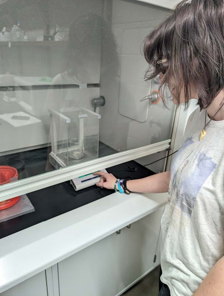
For the first day, we began part one by preparing 4 different test tubes with 10mL of varying concentrations of salt water (distilled water, 1% salt, 3% salt, and 5% salt). Each tube was given 3 cylinders of potato that were each 3 cm long. Prior to being placed into their tubes, each group of potatoes were massed. Since it can take a while to fully observe the effects of osmosis, we left the potatoes in their tubes until the following Monday (Feb. 5). We had some time left on day 1, so we decided to continue onto part 2 of the experiment. For this part, we first observed Elodea cells under a microscope, then we exposed them to a solution of 5% salt water and recorded the changes. Nothing out of the ordinary was viewed until we added the salt water solution, but almost immediately after, the cell membranes began to shrink and pack in all of their organelles. Even though the cell membranes of the Elodea cells shrank, the cell walls remained intact and mostly unchanged.
Wren measuring the weight of potato cores.
On the second day of the experiment we recorded the mass of the potatoes again and noted the change in mass. In the distilled water, the potatoes started with a mass of 3.06g and ended with 1.03g for a change of -2.03g. This change was unexpected and is likely inaccurate due to all the potatoes in the tube losing all structure and becoming a mush. The 1% salt solution potatoes began with a mass of 3.28g and ended with 3.64g for a change of +0.36g. This solution had the most structured potatoes out of all the groups, but it was still a little squishy. In the 3% salt solution, the potatoes began with a mass of 3.20g and ended with 2.53g for a change of -0.67g.
This group of potatoes also retained their shape, but were less structured than the previous group. The group of potatoes were in a 5% salt solution, they began with a mass of 3.71g and ended with 2.99g for a change of -0.72g. The potatoes in this group had a very similar structure to the potatoes in the 3% salt solution group, keeping their structure but still squishy. In the end, we were able to see that the change from a 1% salt to a 3% salt solution was the greatest and rate of change was lower as the concentration increased. It can also be assumed that the cells of the potatoes in the distilled water absorbed too much water and burst through the cell wall, since they lost their structure and became a sludge.
Overall all of the experiments went well, but had some unexpected results. As of right now the only one to sprout in our germination experiment is the common milkweed in germination code E, which is not its natural environment to be grown in. In the potato cores, the zero percent solution cores turned completely to mush while the one percent cores were the most well-maintained shape-wise. We look forward to seeing how our seed germination progresses and the experiments we have coming up.
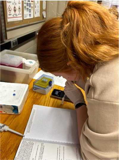
This first month we started practicing pipetting to get more comfortable with lab skills. Then we moved on to PCR and gel electrophoresis. This last week we practiced imaging for the first time, and it went well!
For week one, we focused on our pipetting protocol. We had a lot to learn on proper technique and choosing the right size pipette tip. We used these skills in all the following weeks.
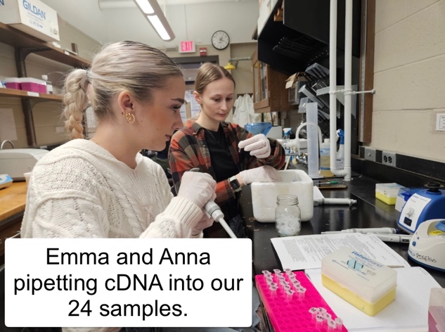
First, we used prepared cDNA samples to run a PCR protocol. We had to calculate the volumes for each step and mix our solution. Then, we vortexed our tubes down making sure to balance the machine for best results. Next, we used our newfound knowledge of pipetting to create positive and negative tests. The positive control contained cDNA, and the negative control contained distilled water. We ran our samples in a thermocycler for approximately two hours before placing the samples in the freezer for future use.
Figure 2: Arya assembling the gel casting tray.
The next week we used our samples for gel electrophoresis. To start we mixed agarose and 1xTAE buffer and microwaved and swirled it until the mixture was clear. We assembled our gel casting tray, adding in the eight-prong comb to create our wells. Our mixture had not cooled all the way, so we ran the flask under cold water until it was warm to the touch. We then added bullseye dye to the agarose mixture. Once this was incorporated, we poured the mixture into the tray, making sure there were no bubbles present. It sat for about 30 minutes to solidify. Once solid, we removed the comb and placed the gel into the machine. There was already some buffer from a previous group, but we topped it off to ensure the gel was completely covered. We pipetted in our ladder, then our positive control, and finally our negative control. For the positive control, the pipette tip broke through the gel. We attempted a second well, but there was not much material left.
The gel ran for about 30 minutes, then we removed it and carried it up to the imager. We placed the gel in the machine following our imaging protocol and properly formatted the image orientation. We took photos of the results for our journals. Our positive control was not successful, but we will try again using what we learned.
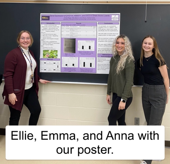
These past two weeks we have been conducting our final experiments on our three genes, ZYG11A, HS6ST1, and DIO2. All the while putting our finishing touches on our final poster for end of the year presentations of our research. DIO2, a gene that we recently added, is a gene that turns deactivated T4 thyroid hormone into activated T3 thyroid hormone. These hormones both play a role in the production of metabolism.
One of the major procedures that we have completed is a standard curve. A standard curve analyzes our NTC (no template control), 5-standard, 1-standard, 0.2-standard, and 0.04-standard tubes. The NTC does not contain cDNA, while the standards contain a specific diluted amount. All of these tubes contain a specific amount of the master mix created. This standard curve run tells us if our standards, as stated, were pipetted properly and accurately. Also, if the cDNA that we used was working and not denatured. This line of samples and our NTC is used as a standard to allow us to compare our 24 cDNA samples and their expression levels.
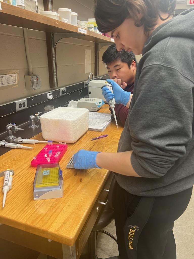
After we received good results for at least one standard curve, we started to run full run qPCRS, or quantitative PCRs. To complete a full run qPCR, we first made Int-1, Int-0.2, and Int-0.04. These all contained water and a diluted amount of cDNA from the previous tube. Next, we created our NTC and standard tubes. We then created a master mix, which contains all of the necessary components to amplify these 24 cDNA samples with the genes forward and reverse primers. Included in the master mix is a liquid called PowerUp SYBR Green 2x Mix. This is the base of the master mix which allows for a lot less area for pipetting error. The rest of the master mix includes both forward and reverse primers and water. This mixture was pipetted into 24 tubes and then the correlating cDNA was added to each of these tubes. These were then pipetted into a 96-well plate and ran through the qPCR machine. Both ZYG11A and HS6ST1 have each had two standard curves and one successful full run qPCR conducted on them and have shown good results. DIO2 had one standard curve and one successful full run qPCR which showed promising results.
After analyzing our results, we concluded that none of our genes had a significant change during the breeding vs non-breeding season in male or female green anole lizards. We created a poster and presented these findings, along with our journey to them, at a poster session this past week. We will be presenting this information again in April at the URS conference on campus.
Since our last blog post in September, we have made significant progress in each of our genes. We also have had great success with the combination of our lab groups. We have found out that we work very well and efficiently together. We had a lot of work that needed to be done, especially early in the semester but we have managed to make good progress in our research especially with the PLD4 gene. Even without progress there is still much to do before the semester is over.
Rebecca performing a PCR cleanup on STAB2 primers with our TA Nick watching.
When it comes to gene progression specifically in PLD4, we designed 3 new primers and found that our new primer set 2 worked very well. The new primer set worked well enough to be able to send for DNA sequencing. Our results came back looking good from the sequencing. During the past few weeks, we were introduced to qPCR reactions. This was a learning curve for us and every other group because we were moving from pipetting into a few tubes to now pipetting into a 96 well plate. We had a lab session where we practiced pipetting into the plate with different colored water to get a feel of what a full run would be like. Our first few qPCRs were not full runs because we were still learning and needed good results on a standard curve to be able to proceed onto the full run. PLD4 looked good in the standard curve runs so we were able to recently complete a full run with PLD4. The full run results came back looking good and when we compared the numbers to beta actin, it supported the hypothesis we originally had made for PLD4 that the inflammatory response will be higher in males during the mating season.
Georgia pipetting our PCR mixes into an agarose gel.
While the work with PLD4 has been going along great, there have been some struggles with STAB2. Initially our STAB2 primers were all set to be run with a qPCR as the primer set we were using had been sequenced last semester and came back looking good. However, we began seeing problems with our standard curve runs of STAB2. The efficiencies of the runs were no where near the value we needed to continue to a full run and when run on a gel would only show primer dimers. We began troubleshooting to see if we needed to alter the conditions of the qPCR to get STAB2 to work. We began with a temperature gradient on a normal PCR and saw that the reaction still worked better at the standard 60℃ but still had primer dimers. Next, we tried the PCR reaction with different primer concentrations to no avail. During our second attempt with primer concentrations, we also made a normal PCR using one of the other two primer sets we created last semester. The other primer set came out well on the PCR so we did a PCR cleanup and sent it out for sequencing. If the sequencing looks right with the other primer set we will make another attempt at running a standard curve with STAB2.
Despite the setbacks with STAB2 we have managed to do well this semester. We were able to get the data needed to test our hypothesis for PLD4 and found that our research supports our hypothesis. We do not yet have the data necessary to do the same for STAB2 but we are making progress to get to that point. This semester has been an excellent experience especially with the opportunity to be working with someone new.
RISEbio is a National Science Foundation funded scholarship program at Minnesota State University, Mankato. This program gives first year students interested in pursuing a degree in biology the opportunity to engage in real-world research with faculty and graduate students.